Formula for sample size proportion

Often sampling is done in order to estimate the proportion of a population that has a specific characteristic, such as the proportion of all items coming off an assembly line that are defective or the proportion of all people entering a retail store who make a purchase before leaving. The population proportion is denoted p and the sample proportion is denoted p ^ . Thus if in reality 43% of people entering a store make a purchase before leaving, p = 0.43; if in a sample of 200 people entering the store, 78 make a purchase, p ^ = 78 / 200 = 0.39 .

The sample proportion is a random variable: it varies from sample to sample in a way that cannot be predicted with certainty. Viewed as a random variable it will be written P ^ . It has a mean The number about which proportions computed from samples of the same size center. μ P ^ and a standard deviation A measure of the variability of proportions computed from samples of the same size. σ P ^ . Here are formulas for their values.

Suppose random samples of size n are drawn from a population in which the proportion with a characteristic of interest is p. The mean μ P ^ and standard deviation σ P ^ of the sample proportion P ^ satisfy

μ P ^ = p and σ P ^ = p q n

The Central Limit Theorem has an analogue for the population proportion P ^ . To see how, imagine that every element of the population that has the characteristic of interest is labeled with a 1, and that every element that does not is labeled with a 0. This gives a numerical population consisting entirely of zeros and ones. Clearly the proportion of the population with the special characteristic is the proportion of the numerical population that are ones; in symbols,

p = number of 1 s N

But of course the sum of all the zeros and ones is simply the number of ones, so the mean μ of the numerical population is

μ = Σ x N = number of 1 s N

Thus the population proportion p is the same as the mean μ of the corresponding population of zeros and ones. In the same way the sample proportion p ^ is the same as the sample mean x - . Thus the Central Limit Theorem applies to P ^ . However, the condition that the sample be large is a little more complicated than just being of size at least 30.

The Sampling Distribution of the Sample Proportion

For large samples, the sample proportion is approximately normally distributed, with mean μ P ^ = p and standard deviation σ P ^ = p q / n .

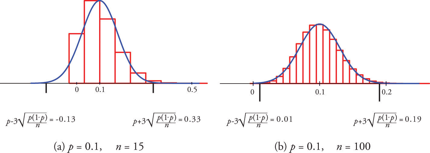
A sample is large if the interval [ p − 3 σ P ^ , p + 3 σ P ^ ] lies wholly within the interval [ 0,1 ] .

In actual practice p is not known, hence neither is σ P ^ . In that case in order to check that the sample is sufficiently large we substitute the known quantity p ^ for p. This means checking that the interval

[ p ^ − 3 p ^ ( 1 − p ^ ) n , p ^ + 3 p ^ ( 1 − p ^ ) n ]

lies wholly within the interval [ 0,1 ] . This is illustrated in the examples.

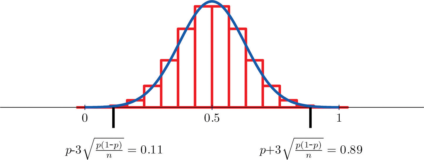
Figure 6.5 "Distribution of Sample Proportions" shows that when p = 0.1 a sample of size 15 is too small but a sample of size 100 is acceptable. Figure 6.6 "Distribution of Sample Proportions for " shows that when p = 0.5 a sample of size 15 is acceptable.

Figure 6.5 Distribution of Sample Proportions

Figure 6.6 Distribution of Sample Proportions for p = 0.5 and n = 15

Example 7

Suppose that in a population of voters in a certain region 38% are in favor of particular bond issue. Nine hundred randomly selected voters are asked if they favor the bond issue.

Verify that the sample proportion P ^ computed from samples of size 900 meets the condition that its sampling distribution be approximately normal.
Find the probability that the sample proportion computed from a sample of size 900 will be within 5 percentage points of the true population proportion.

The information given is that p = 0.38, hence q = 1 − p = 0.62 . First we use the formulas to compute the mean and standard deviation of P ^ : μ P ^ = p = 0.38 and σ P ^ = p q n = ( 0.38 ) ( 0.62 ) 900 = 0.01618 Then 3 σ P ^ = 3 ( 0.01618 ) = 0.04854 ≈ 0.05 so [ p − 3 σ P ^ , p + 3 σ P ^ ] = [ 0.38 − 0 . 05,0 . 38 + 0.05 ] = [ 0 . 33,0 . 43 ] which lies wholly within the interval [ 0,1 ] , so it is safe to assume that P ^ is approximately normally distributed.
To be within 5 percentage points of the true population proportion 0.38 means to be between 0.38 − 0.05 = 0.33 and 0.38 + 0.05 = 0.43 . Thus P ( 0.33 < P ^ < 0.43 ) = P ( 0.33 − μ P ^ σ P ^ < Z < 0.43 − μ P ^ σ P ^ ) = P ( 0.33 − 0.38 0.01618 < Z < 0.43 − 0.38 0.01618 ) = P ( − 3.09 < Z < 3.09 ) = P ( 3.09 ) − P ( − 3.09 ) = 0.9990 − 0.0010 = 0.9980

Example 8

An online retailer claims that 90% of all orders are shipped within 12 hours of being received. A consumer group placed 121 orders of different sizes and at different times of day; 102 orders were shipped within 12 hours.

Compute the sample proportion of items shipped within 12 hours.
Confirm that the sample is large enough to assume that the sample proportion is normally distributed. Use p = 0.90, corresponding to the assumption that the retailer’s claim is valid.
Assuming the retailer’s claim is true, find the probability that a sample of size 121 would produce a sample proportion so low as was observed in this sample.
Based on the answer to part (c), draw a conclusion about the retailer’s claim.

The sample proportion is the number x of orders that are shipped within 12 hours divided by the number n of orders in the sample: p ^ = x n = 102 121 = 0.84
Since p = 0.90, q = 1 − p = 0.10 , and n = 121, σ P ^ = ( 0.90 ) ( 0.10 ) 121 = 0.0 27 - hence [ p − 3 σ P ^ , p + 3 σ P ^ ] = [ 0.90 − 0 . 08,0 . 90 + 0.08 ] = [ 0 . 82,0 . 98 ] Because [ 0.82 , 0.98 ] ⊂ [ 0,1 ] , it is appropriate to use the normal distribution to compute probabilities related to the sample proportion P ^ .
Using the value of P ^ from part (a) and the computation in part (b), P ( P ^ ≤ 0.84 ) = P ( Z ≤ 0.84 − μ P ^ σ P ^ ) = P ( Z ≤ 0.84 − 0.90 0.0 27 - ) = P ( Z ≤ − 2.20 ) = 0.0139
The computation shows that a random sample of size 121 has only about a 1.4% chance of producing a sample proportion as the one that was observed, p ^ = 0.84 , when taken from a population in which the actual proportion is 0.90. This is so unlikely that it is reasonable to conclude that the actual value of p is less than the 90% claimed.

Key Takeaways

The sample proportion is a random variable P ^ .
There are formulas for the mean μ P ^ and standard deviation σ P ^ of the sample proportion.
When the sample size is large the sample proportion is normally distributed.

Exercises

Basic

The proportion of a population with a characteristic of interest is p = 0.37. Find the mean and standard deviation of the sample proportion P ^ obtained from random samples of size 1,600.

The proportion of a population with a characteristic of interest is p = 0.82. Find the mean and standard deviation of the sample proportion P ^ obtained from random samples of size 900.

The proportion of a population with a characteristic of interest is p = 0.76. Find the mean and standard deviation of the sample proportion P ^ obtained from random samples of size 1,200.

The proportion of a population with a characteristic of interest is p = 0.37. Find the mean and standard deviation of the sample proportion P ^ obtained from random samples of size 125.

Random samples of size 225 are drawn from a population in which the proportion with the characteristic of interest is 0.25. Decide whether or not the sample size is large enough to assume that the sample proportion P ^ is normally distributed.

Random samples of size 1,600 are drawn from a population in which the proportion with the characteristic of interest is 0.05. Decide whether or not the sample size is large enough to assume that the sample proportion P ^ is normally distributed.

n = 50, p ^ = 0.48
n = 50, p ^ = 0.12
n = 100, p ^ = 0.12

n = 30, p ^ = 0.72
n = 30, p ^ = 0.84
n = 75, p ^ = 0.84

P ( 0.45 ≤ P ^ ≤ 0.50 )
P ( P ^ ≥ 0.50 )

P ( 0.25 ≤ P ^ ≤ 0.40 )
P ( P ^ ≤ 0.35 )

P ( 0.60 ≤ P ^ ≤ 0.64 )
P ( 0.57 ≤ P ^ ≤ 0.67 )

P ( 0.27 ≤ P ^ ≤ 0.29 )
P ( 0.23 ≤ P ^ ≤ 0.33 )

Applications

Suppose that 8% of all males suffer some form of color blindness. Find the probability that in a random sample of 250 men at least 10% will suffer some form of color blindness. First verify that the sample is sufficiently large to use the normal distribution.

Suppose that 29% of all residents of a community favor annexation by a nearby municipality. Find the probability that in a random sample of 50 residents at least 35% will favor annexation. First verify that the sample is sufficiently large to use the normal distribution.

Suppose that 2% of all cell phone connections by a certain provider are dropped. Find the probability that in a random sample of 1,500 calls at most 40 will be dropped. First verify that the sample is sufficiently large to use the normal distribution.

Suppose that in 20% of all traffic accidents involving an injury, driver distraction in some form (for example, changing a radio station or texting) is a factor. Find the probability that in a random sample of 275 such accidents between 15% and 25% involve driver distraction in some form. First verify that the sample is sufficiently large to use the normal distribution.

Compute the sample proportion.
Assuming the airline’s claim is true, find the probability of a sample of size 30 producing a sample proportion so low as was observed in this sample.

A humane society reports that 19% of all pet dogs were adopted from an animal shelter. Assuming the truth of this assertion, find the probability that in a random sample of 80 pet dogs, between 15% and 20% were adopted from a shelter. You may assume that the normal distribution applies.

In one study it was found that 86% of all homes have a functional smoke detector. Suppose this proportion is valid for all homes. Find the probability that in a random sample of 600 homes, between 80% and 90% will have a functional smoke detector. You may assume that the normal distribution applies.

A state insurance commission estimates that 13% of all motorists in its state are uninsured. Suppose this proportion is valid. Find the probability that in a random sample of 50 motorists, at least 5 will be uninsured. You may assume that the normal distribution applies.

An outside financial auditor has observed that about 4% of all documents he examines contain an error of some sort. Assuming this proportion to be accurate, find the probability that a random sample of 700 documents will contain at least 30 with some sort of error. You may assume that the normal distribution applies.

Suppose 7% of all households have no home telephone but depend completely on cell phones. Find the probability that in a random sample of 450 households, between 25 and 35 will have no home telephone. You may assume that the normal distribution applies.

Additional Exercises

Some countries allow individual packages of prepackaged goods to weigh less than what is stated on the package, subject to certain conditions, such as the average of all packages being the stated weight or greater. Suppose that one requirement is that at most 4% of all packages marked 500 grams can weigh less than 490 grams. Assuming that a product actually meets this requirement, find the probability that in a random sample of 150 such packages the proportion weighing less than 490 grams is at least 3%. You may assume that the normal distribution applies.

Find the sample proportion.
Find the probability that, when a sample of size 325 is drawn from a population in which the true proportion is 0.38, the sample proportion will be as large as the value you computed in part (a). You may assume that the normal distribution applies.
Give an interpretation of the result in part (b). Is there strong evidence that people are keeping their cars longer than was the case five years ago?

Find the sample proportion.
Find the probability that, when a sample of size 1,500 is drawn from a population in which the true proportion is 0.22, the sample proportion will be no larger than the value you computed in part (a). You may assume that the normal distribution applies.
Give an interpretation of the result in part (b). How strong is the evidence that the campaign to reduce smoking has been effective?

What information is missing that you would need to compute the probability that a sample drawn from a population in which the proportion is 78% (corresponding to the assumption that the low-cost clinic had had no effect) is as high as 86%?
Knowing that the size of the original sample three years ago was 150 and that the size of the recent sample was 125, compute the probability mentioned in part (a). You may assume that the normal distribution applies.
Give an interpretation of the result in part (b). How strong is the evidence that the presence of the low-cost clinic has increased the proportion of pet dogs and cats that have been spayed or neutered?

Find the probability that a fair die would produce a proportion of 0.15 or less. You may assume that the normal distribution applies.
Give an interpretation of the result in part (b). How strong is the evidence that the die is not fair?
Suppose the sample proportion 0.15 came from rolling the die 2,400 times instead of only 240 times. Rework part (a) under these circumstances.
Give an interpretation of the result in part (c). How strong is the evidence that the die is not fair?